Power BI: Calculation from two tables


Maximum Analytical Performance: Power BI and the Art of Table Relationships
In the world of data analysis, Power BI is a vital tool that enables the visualization and analysis of complex data relationships. A key aspect of this is the ability to perform calculations across multiple tables. In this blog post, we dive into the fundamentals of table relationships in Power BI, explain the use of RELATED and RELATEDTABLE for data queries, and provide practical examples and best practices for efficient data models.
Fundamentals of Table Relationships in Power BI
Table relationships in Power BI are more than just connections between data points—they are the foundation upon which meaningful and interactive data models are built. These relationships allow analysts to integrate, analyze, and visualize complex data from various sources. To fully understand the significance and mechanics of these relationships, it is essential to know their basics and types.
Primary Keys and Foreign Keys: The Core of Relationships
The primary key is a unique identifier in a table. Every record in that table can be uniquely identified by its primary key. A clear example of this is a Customer ID in a customer table, where each ID is assigned to a specific customer.
The foreign key refers to the primary key in another table, thereby serving as a link between the tables. For example, an orders table might contain a Customer ID as a foreign key that points to the primary key in the customer table.
Different Types of Relationships
Data relationships are at the heart of many BI tools. These relationships allow us to link complex data from different sources and gain meaningful insights into our business processes. In Power BI, relationship types play a crucial role as they determine how data from different tables interact and are interpreted. Below, we will take a closer look at the various relationship types in Power BI and explain how they impact data analysis and reporting.
Power BI distinguishes between four different relationship types, which define how tables relate to one another.
One-to-One (1:1) means that each record in the first table corresponds to exactly one record in the second table. This relationship type is rare, as it requires both tables to contain unique records.
One-to-Many (1:N) is the most common relationship type. In this case, one record in the first table (containing the primary key) corresponds to multiple records in the second table. An example would be a relationship between a product information table (where each product is unique) and a sales table, where each product can be sold multiple times. (See Figure 1)
Many-to-One (N:1) is essentially the reverse perspective of a 1:N relationship. Here, multiple records in the first table correspond to a single record in the second table.
Many-to-Many (M:N) represents a relationship where multiple rows from the first table belong to multiple rows from the second table. This type occurs, for example, when multiple products can be sourced from multiple suppliers, and each supplier in turn provides multiple products. This relationship can lead to challenges and calculation errors in data models. It is therefore recommended to avoid this relationship whenever possible.

Using RELATED and RELATEDTABLE
The RELATED and RELATEDTABLE functions in Power BI are essential tools for working with relational data models. They allow you to efficiently query and analyze data from different, yet interconnected, tables. To fully understand their application and significance, it is helpful to take a closer look at each function and its potential use cases.
RELATED: Accessing linked data
The RELATED function is used in Power BI to access values from another table that is connected via a relationship. It plays a crucial role in data modeling and analysis, particularly in "one-to-many" and "many-to-one" relationships.
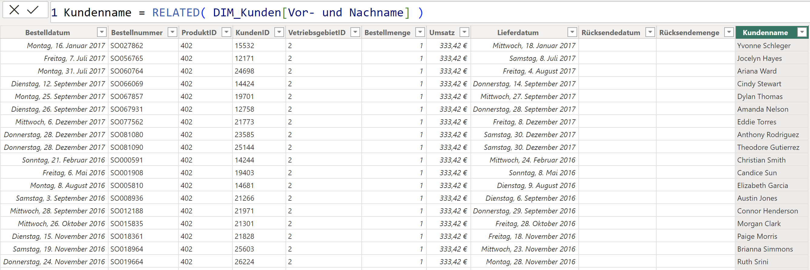
Application example: Suppose you have a table with sales data (Sales table) and a separate table with customer information (DIM_Customers). Each sale is assigned to an employee. To display the employee's name in the sales table, you can use the RELATED function to retrieve the name from the employee table based on the employee ID. In DAX (Data Analysis Expressions), the formula might look like this: CustomerName = RELATED(DIM_Customers[First and Last Name]). This formula would be used in the sales table to extract the employee's name from the employee table.
RELATEDTABLE: Summarizing data from related tables
RELATEDTABLE is a powerful function that returns a table of values from a related table. It is frequently used in "one-to-many" relationships to calculate summarized data such as totals, averages, or counts.
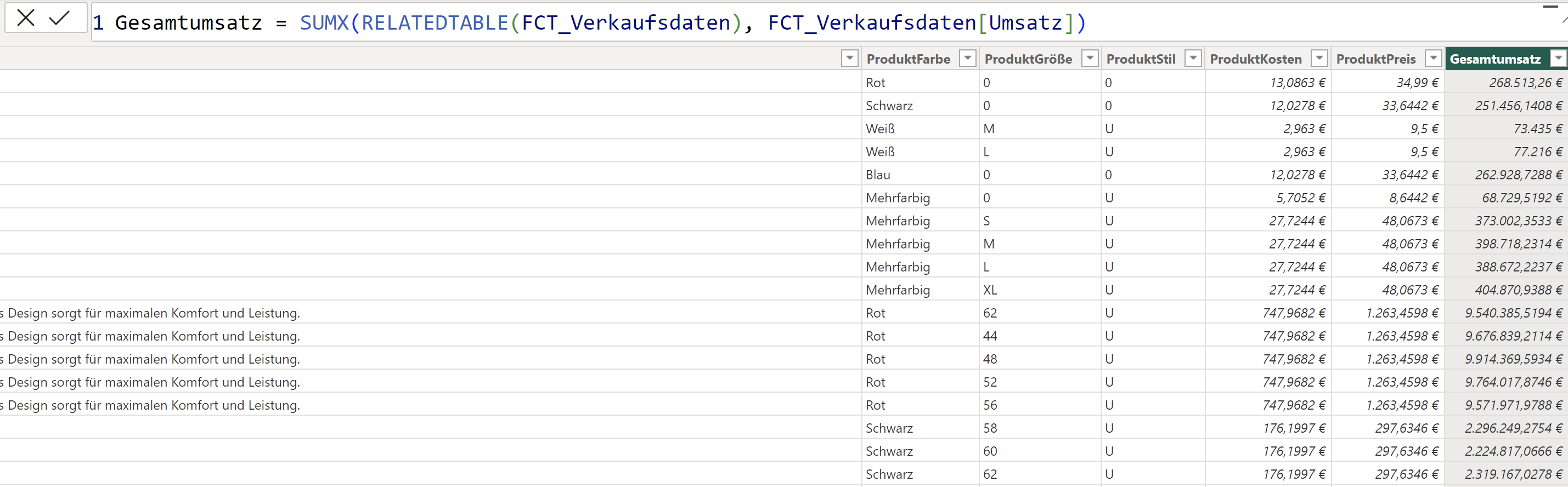
Application example: Imagine you have a table with product information (Product table) and a table with sales data (FCT_SalesData), where each product can be sold multiple times. To calculate the total revenue per product, you can use the RELATEDTABLE function to summarize all sales for a specific product. A typical DAX formula might look like this: TotalRevenue = SUMX(RELATEDTABLE(FCT_SalesData), FCT_SalesData[Revenue]). This formula would be used in the product table to calculate the total revenue for each product based on the data in the sales table.
For the effective use of these functions, it is crucial that the relationships between the tables are correctly defined. Incorrectly defined relationships can lead to inaccurate results. It should also be noted that RELATED can only be used in calculated columns or measure formulas, while RELATEDTABLE is typically used in measure formulas.
Examples of common scenarios for calculations across two tables in Power BI
Applying RELATED and RELATEDTABLE in Power BI opens up a multitude of possibilities for detailed and insightful data analysis. A particularly clear example is calculating revenue across multiple tables. To illustrate the practical application of these functions, let's look at an advanced scenario involving sales data and product information.
Scenario: Sales analysis using sales and product data
Imagine you have two main tables in your Power BI model.
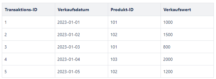
- Sales table: This table contains detailed sales data, including transaction IDs, sales dates, product IDs, and sales values.
Example sales table:
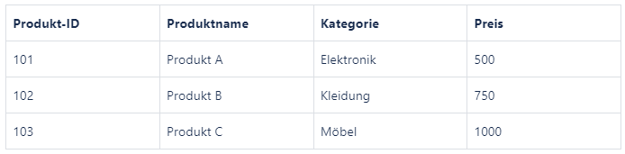
- Product table: This table lists all products with product IDs, product descriptions, categories, and prices.
Example product table:
The goal is to create a comprehensive analysis of revenue that takes into account not only sales figures but also product information.
Using RELATED: Detailed product information in sales reports
- The problem: You have the product ID in the sales table, but no further information about the product.
- The solution: You can use the RELATED function to pull product details such as the name, category, or price from the product table into the sales table.
- Example: Product Name = RELATED(ProductTable[ProductName])
-
This formula is applied in the sales table to retrieve the product name based on the product ID. The result in your sales report would look like this:

Using the RELATED function pulls product information from the product table into the sales table, making your sales reports more informative.
Using RELATEDTABLE: Aggregating total sales by product
- The challenge: You want to determine the total sales per product or category, but the sales table only contains individual transactions.
- The solution: RELATEDTABLE allows you to aggregate all relevant sales data for each product to calculate total revenue.
- Example: To calculate total sales per product, you can use the RELATEDTABLE function. Here is an example formula in Power BI: TotalSalesProduct = SUMX(RELATEDTABLE(SalesTable), SalesTable[Revenue])
This formula in the product table calculates the total revenue for each product by aggregating all sales from the sales table. The result in your product table would look like this:
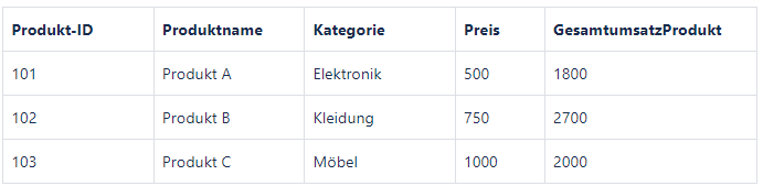
Using the RELATEDTABLE function aggregates all sales data from the sales table to calculate total revenue per product. This enables a detailed analysis of revenue for each individual product.
Best practices for efficient data models in Power BI
Efficient data models are the heart of powerful analytics in Power BI. They determine not only the accuracy and relevance of your analysis results but also the speed and efficiency with which those results are achieved. Here are some advanced best practices for creating and maintaining efficient, high-performance data models in Power BI.
A clear and logical structuring of relationships between tables is crucial for the integrity and performance of the data model. It is important to accurately identify primary and foreign key relationships and to avoid redundant or circular relationships.
Another important approach is the use of the star schema. This data modeling principle, in which a central fact table is surrounded by multiple dimension tables, simplifies data querying and analysis. It offers an intuitive and clear structure and improves performance, as fewer joins are required. Organizing data by storing transaction data in the fact table and descriptive attributes in the dimension tables is essential here.
The optimization of data through data cleansing also contributes to increased efficiency. Simpler and less complex DAX formulas are often more efficient and easier to maintain. In addition, you should consider how often data needs to be refreshed, as frequent updates, especially with large volumes of data, can impair performance. Furthermore, regular review and maintenance of the data model is essential. Performance bottlenecks can be identified through performance monitoring, for example using the Performance Analyzer in Power BI. If business requirements change, the model should be adjusted accordingly.
An efficient data model in Power BI is the result of careful planning, smart structuring, and regular maintenance.